
Correlation & Regression: Compare models; transform — TJC 2025 H2 Math Prelim Paper 2
What this question tests
Question
Anand signed up for a privilege card with Temasek Airlines where cardholders earn more reward points as they fly further with the airline. From the airlines' website, Anand identified 8 different destinations and recorded the flight distance, \(x\) miles, of each destination from Singapore. He also recorded the corresponding reward points, \(y\), credited into his card after each flight. The data are shown below.
| Destination | A | B | C | D | E | F | G | H |
|---|---|---|---|---|---|---|---|---|
| Flight distance, \(x\) | 200 | 400 | 600 | 800 | 1000 | 1200 | 1400 | 1600 |
| Reward points, \(y\) | 110 | 160 | 190 | 200 | 210 | 215 | 220 | 225 |
- Sketch a scatter diagram of the data.
- Calculate the value of the product moment correlation coefficient, and explain why this value does not necessarily mean that a linear model is the best for the relationship between \(x\) and \(y\).
- Without calculating the product moment correlation coefficient, explain which of the following equations, where \(a\) and \(b\) are constants, and \(b > 0\), can be used to model the relationship between \(x\) and \(y\). \[\begin{aligned} \text{(I)} &\quad y = a + bx^2\\ \text{(II)} &\quad y = a + b\ln x\\ \text{(III)} &\quad y = a + b\mathrm{e}^{-x} \end{aligned}\]
- Using the model identified in (c), find the equation of the corresponding regression line.
- Hence estimate the reward points that can be earned for a destination 700 miles away from Singapore. Comment on the reliability of your estimation.
- It is given that 1 mile is approximately 1.609 kilometres. State what will happen to the product moment correlation coefficient found in (b) if the flight distance is measured in kilometres instead of miles.
Show full worked solution▾
(a) Scatter diagram:
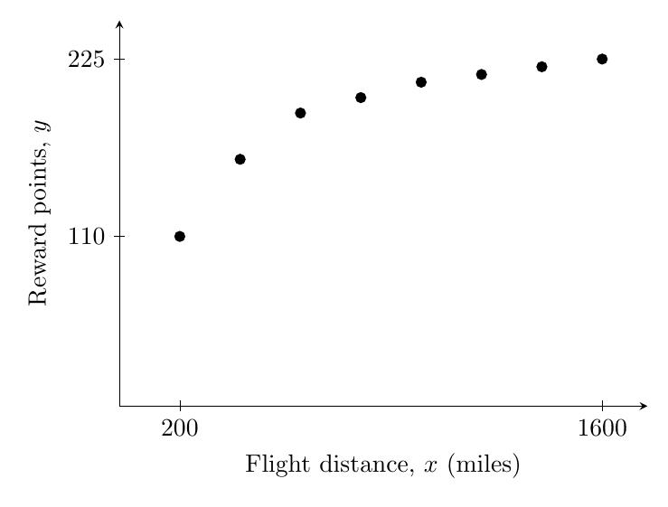
(b) From GC: \(r = 0.894\) (3 s.f.).
Even though the \(r\)-value indicates a strong positive linear correlation between \(x\) and \(y\), the scatter diagram shows that the data follows a curvilinear (concave downward) pattern. Therefore a linear model may not be the best for the relationship.
(c) Analysing each model with \(b>0\):
Model I (\(y = a+bx^2\)): As \(x\) increases, \(x^2\) increases at an increasing rate, so \(y\) would increase at an increasing rate. This does not match the scatter diagram (increasing at a decreasing rate). Not suitable.
Model II (\(y = a+b\ln x\)): As \(x\) increases, \(\ln x\) increases at a decreasing rate (concave down), so \(y\) increases at a decreasing rate. This matches the scatter diagram. Suitable.
Model III (\(y = a+b\mathrm{e}^{-x}\)): With \(b>0\) and \(\mathrm{e}^{-x}\) decreasing, \(y\) would decrease as \(x\) increases. This does not match. Not suitable.
Hence Model II (\(y = a+b\ln x\)) is the best model.
(d) Using GC, the regression line of \(y\) on \(\ln x\) is: \[y = 54.269\ln x - 168.22\] i.e. \(y = 54.3\ln x - 168\) (3 s.f.).
(e) When \(x = 700\): \[y = 54.269\ln 700 - 168.22 = 54.269\times 6.5511 - 168.22 = 355.54 - 168.22 \approx 187\ \text{(3 s.f.)}\]
The input \(x = 700\) lies within the data range \([200, 1600]\), so the estimation is an interpolation. Furthermore, \(r = 0.984\) for \(y\) on \(\ln x\) indicates a very strong positive linear correlation. Therefore the estimation is reliable.
(f) The product moment correlation coefficient between \(x\) and \(y\) measures the linear association between them. Changing the unit of \(x\) from miles to kilometres is a linear scaling (\(x_\text{km} = 1.609x\)), which does not affect the correlation coefficient.